Chicago Voting Data Analysis

Voting fraud and Benford’s law:

I wanted to replicate a few of the plots created in this video about Benford’s Law and voting fraud. I’m doing this mostly because it is fun, and because I want my research students to try it too. I’m not a political scientist, and I’ll leave the interpretation of these data to experts. To summarize the point of the video, I quote the following passage from Deckert et.al. (2011):

“Benford’s Law is problematical at best as a forensic tool when applied to elections.”

On to the video

I will copy a few of the experts pointed out in the video to this page too. If you want an expert viewpoint, start there.

• Check out Steve Mould’s Numberphile video about Benford’s Law.
• There’s more on Mark Nigrini’s work here:
• “Benford’s Law and the Detection of Election Fraud” 2011 paper. (Requires access to this journal. ECU has access as of the date of this writing.)
• And for balance, here is a paper critical of that other paper (but only in the use of a ‘second digit’ check and they do not dispute the main Benford’s Law claims.).
• And here is a paper by the same author specifically about the 2020 US election results

What is Benford’s law?

Benford’s law states that the probability that the first digit of data that spans multiple orders of magnitude follows the following probability distribution: \(P(d) = \log\left(1+\frac{1}{d}\right)\) We are going to look at that with voting data in Chicago.

Dataset

These data were obtained from the Chicago Board of Election commisioners website.

I cleaned this data elsewhere and saved the voteTally object to this file:

load('chicagoVoteTally.RData')

Presidential candidates who were on the ballot in Chicago were:

• Joe Biden (Democrat)
• Donald Trump (Republican)
• Howie Hawkins (Green)
• Gloria La Riva (Party for Socialism and Liberation)
• Brian Carroll (American Solidarity Party)
• Jo Jorgensen (Libertarian)

The 3rd party candidates were not included in Parker’s video, but I thought it might be fun to include them.

The following functions will be used to process the data further:

firstDigit = function(x){
    # Returns the first non-zero digit of any number.  
    # It assumes the number is greater than 0.
    if(!x>=0){
        stop("Number must be greater than or equal to zero")
    }
    x = as.character(x)
    firstX = unlist(strsplit(x,split=''))[1]
    firstX = as.numeric(firstX)
    return(firstX)
}

last2digits = function(x){
    ## Turn x into a character
    x = as.character(x)
    ## Split the character into all the characters
    splitX = unlist(strsplit(x,split=''))
    ## Figure out how many digits you have
    d = length(splitX)
    if(d==1){
        last2X = paste0("0",splitX)
    }else{
        ## Grab last two digits
        last2X = splitX[(d-1):d]
        last2X = paste0(last2X,collapse='')
    }
    return(last2X)
}

drawBenfordPlot = function(dat,candidate,barColor,curveColor='gold'){
    ## If any precincts have zero votes for a candidate, remove them
    dat = dat[dat!=0]
    ## Get the first digits
    dat = sapply(dat,FUN=firstDigit)
    ymaxBen = 1.1*length(dat)*log10(2)
    ymax = max(c(ymaxBen,1.1*max(table(dat))))
    ttl = paste(candidate,'Vote First Digit')
    hist(dat, xlab="First Digit", main=ttl, col=barColor,breaks=0:9,
                   ylim=c(0,ymax), axes=F)
    axis(side=1, at=seq(0.5,8.5,by=1), labels=1:9)
    axis(2)
    # What does Benford's law say should be the answer.  Overlay as a curve
    x = 1:9 
    benford = length(dat) * log10(1+1/x)
    lines(x-0.5,benford,col=curveColor,lwd=3)
}

drawLastTwoDigitPlot = function(dat,candidate,barColor){
    ## Get the last two digits
    dat = sapply(dat,FUN = last2digits)
    counts = table(dat)
    ## Make a title and plot
    ttl = paste(candidate,'Vote Last Two digit pairs')
    barplot(counts, xlab="Last Two Digits", main=ttl, col=barColor)
}

Biden plots

drawBenfordPlot(dat=voteTally$BidenVotes,candidate = "Biden", barColor = 'blue')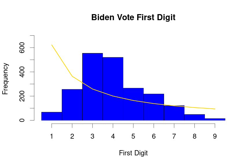

drawLastTwoDigitPlot(dat=voteTally$BidenVotes,candidate="Biden",barColor="blue")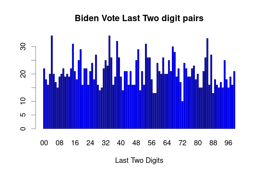

Trump plots

drawBenfordPlot(dat=voteTally$TrumpVotes,candidate = "Trump", barColor = 'red')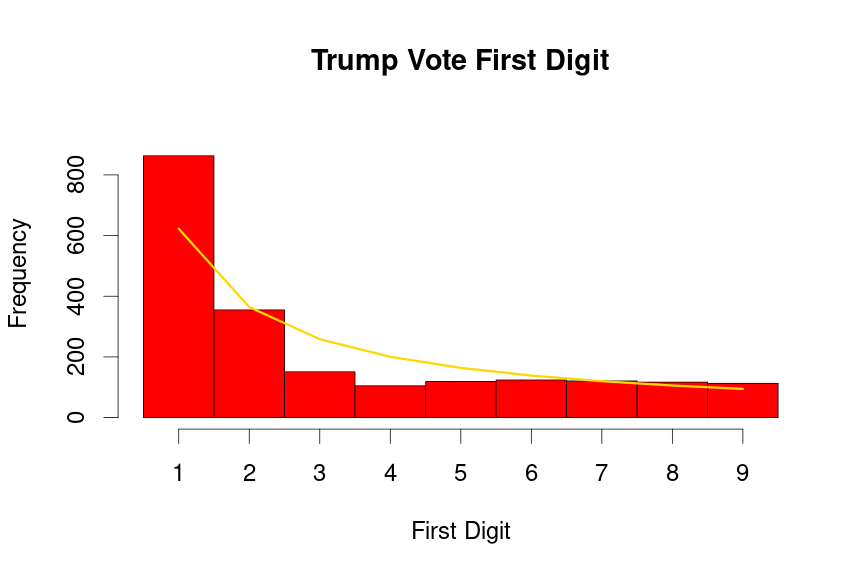

drawLastTwoDigitPlot(dat=voteTally$TrumpVotes,candidate="Trump",barColor="red")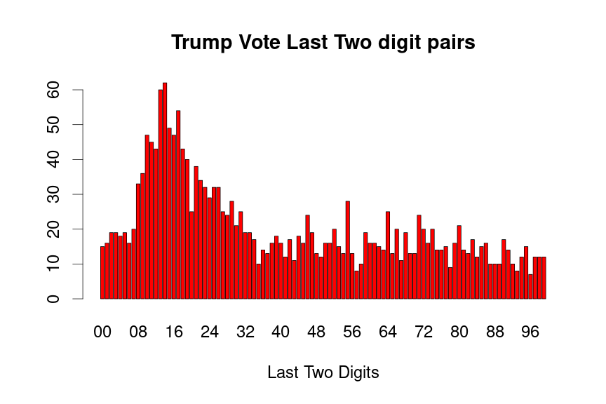

“Third party” candidates

Parker didn’t include so-called third party candidates, but I didn’t want to leave them out. Granted the total votes for these candidates were quite small. Here is a histogram of all of the precinct vote distributions. (No pretty colors because I’m lazy)

voteTotals = voteTally[ ,c(4,6,8,10,12,14)]
library(Hmisc)
hist.data.frame(voteTotals)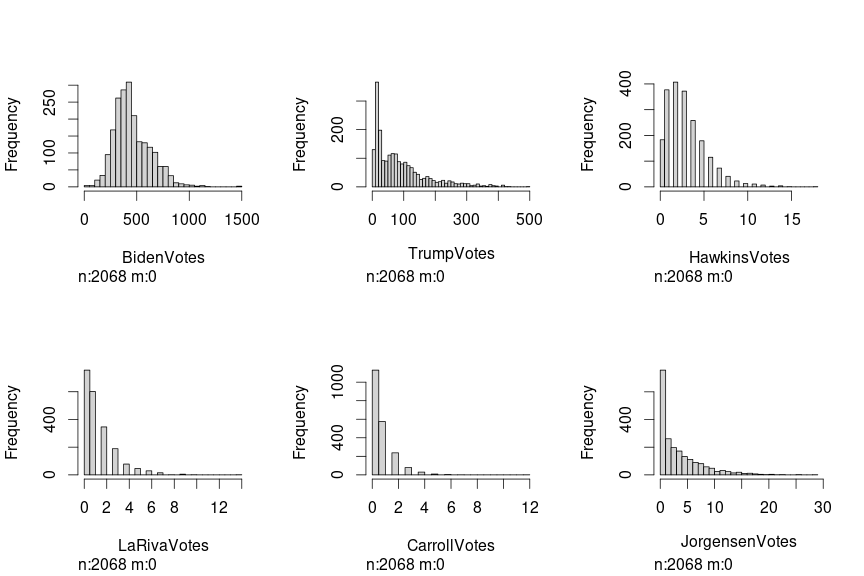

Hawkins plots

drawBenfordPlot(dat=voteTally$HawkinsVotes,candidate = "Hawkins", barColor = 'green')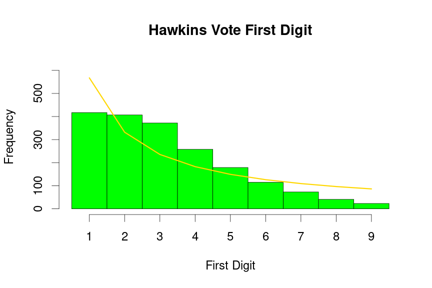

drawLastTwoDigitPlot(dat=voteTally$HawkinsVotes,candidate="Hawkins",barColor="green")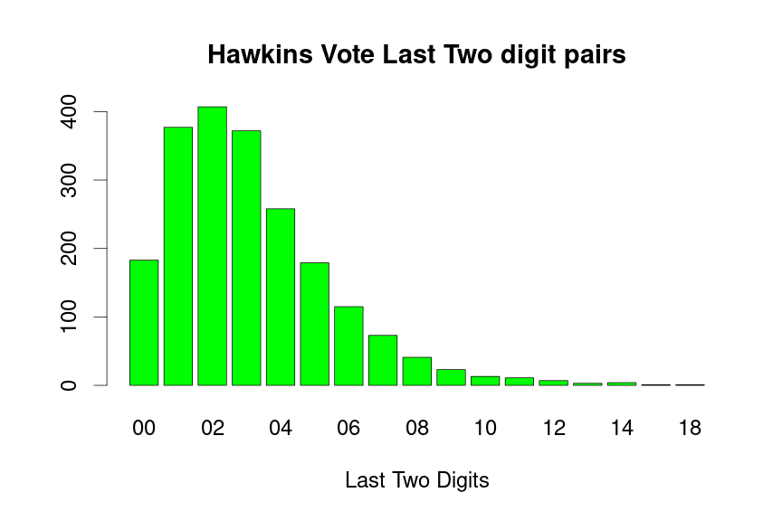

La Riva plots

drawBenfordPlot(dat=voteTally$LaRivaVotes,candidate = "La Riva", barColor = 'purple')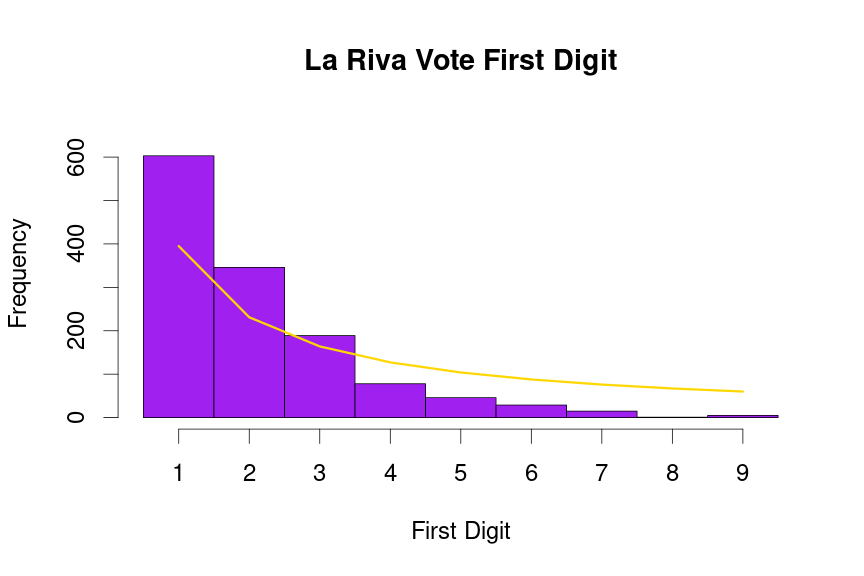

drawLastTwoDigitPlot(dat=voteTally$LaRivaVotes,candidate="La Riva",barColor="purple")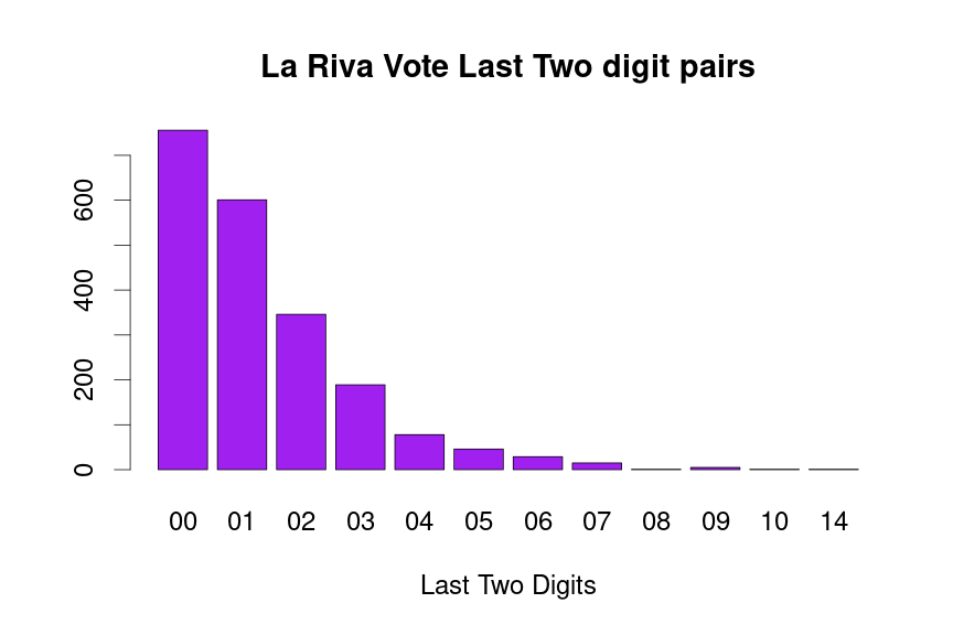

Carroll plots

drawBenfordPlot(dat=voteTally$CarrollVotes,candidate = "Carroll", barColor = 'lightgray')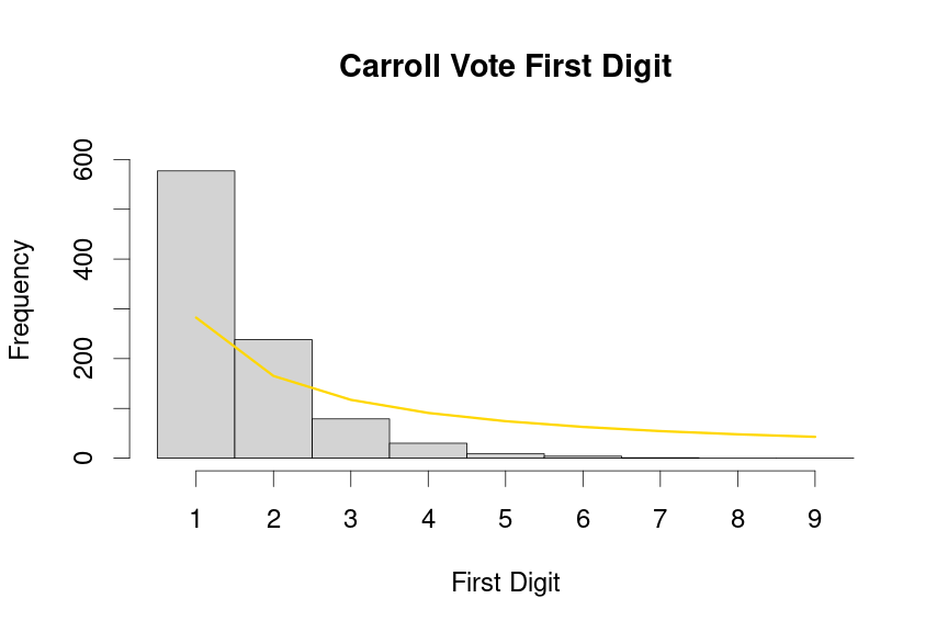

drawLastTwoDigitPlot(dat=voteTally$CarrollVotes,candidate="Carroll",barColor="lightgray")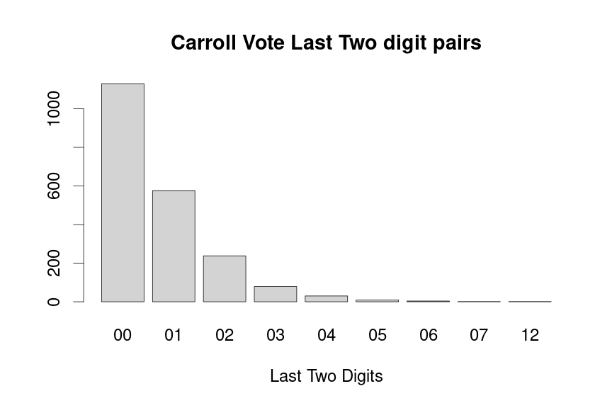

Jorgensen plots

drawBenfordPlot(dat=voteTally$JorgensenVotes,candidate = "Jorgensen", barColor = 'gold',
                curveColor='black')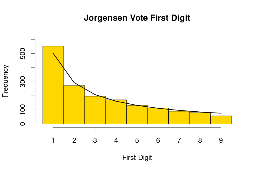

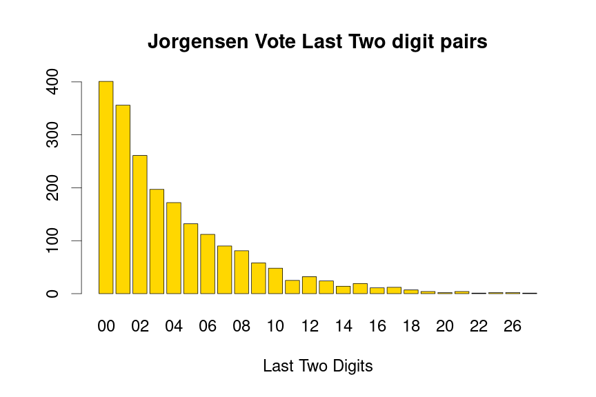
drawLastTwoDigitPlot(dat=voteTally$JorgensenVotes,candidate="Jorgensen",barColor="gold")